Gradient-Based Optimization for Large Systems
Introduction to MDO Architectures, Solvers, and Simulators
Multidisciplinary Design Optimization Architecture
A computational architecture for Multidisciplinary Design Optimization (MDO) is composed of three primary components: solvers (e.g., Newton), simulators (or emulators, PDE solvers, closed-form expressions), and optimizers (e.g., IPOPT, Genetic Algorithm). The performance and efficiency of the overall system are directly influenced by the selection and interaction of these components.
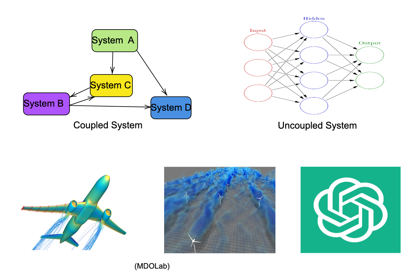
Simulators and solvers are required to either compute the performance of the system through some physics (numerical simulation) or resolve non-linear feedback coupling between subsystems (non-linear equation solvers). A system where all the subsystems agree on their input and output (including any shared variables) is necessary for the system to be optimal and feasible. The coordination of the variables can, however, be done in numerous ways that involve solvers and/or optimizers. Many architectures that arise due to these choices are briefly discussed in later sections.
For offshore systems, marine hydrodynamics solvers (like the boundary element method) are required. The choice of solvers, however, depends on the strength of the coupling between two subsystems. In this post, a Newton solver is used to converge the feedback coupling when necessary.
MDO ‘Stack’
The MDO system can be represented as a set:
\[F:\{\mathcal{O}, \mathcal{M}, \mathcal{S}\}\]
where \(\mathcal{M}\) is the set of simulators, \(\mathcal{O}\) is the choice of optimizer, and \(\mathcal{S}\) is the set of solvers.
The performance \(\mathcal{P}(\mathcal{F})\) depends on:
- The compatibility of \(\mathcal{M}\) and \(\mathcal{S}\) with \(\mathcal{O}\).
- The computational efficiency of \(\mathcal{F}\), defined by the time \(T(\mathcal{F})\) and accuracy \(A(\mathcal{F})\).
- The convergence of the optimization problem.
Gradient-based optimizers (\(\mathcal{O}_{\nabla}\)) achieve superior performance (\(\mathcal{P}(\mathcal{F}_{\nabla}) > \mathcal{P}(\mathcal{F}_{\neg \nabla})\)) when \(\mathcal{M}\) and \(\mathcal{S}\) are differentiable. However, the practical challenges of computing gradients for certain simulators and solvers remain a significant limitation.
Choice of Optimizer
Let \(\mathcal{F}\) represent the multidisciplinary optimization problem, where each problem \(p \in \mathcal{F}\) is defined by a set of variables (design, shared, target), constraints (including consistency constraints), and objectives (one or many). The optimizer is a function \(\mathcal{O}: \mathcal{F} \to \mathcal{R}\), where \(\mathcal{R}\) is the space of feasible solutions.
Optimizers commonly used in MDO problems can be broadly categorized into:
- Gradient-Based Optimizers (\(\mathcal{O}_{\nabla}\)): These optimizers leverage the gradient \(\nabla f\) of the objective function \(f\) to iteratively find a minimum. The preference for gradient-based methods arises from their superior convergence speed when gradients are available and computationally inexpensive. However, obtaining gradients can be challenging:
- Certain simulator software \(S: \mathcal{X} \to \mathcal{Y}\), where \(\mathcal{X}\) is the input space and \(\mathcal{Y}\) is the output space, may not inherently provide differentiable mappings.
- Numerical approximations such as finite differences (\(\nabla f \approx \frac{\Delta f}{\Delta x}\)) may introduce errors and computational overhead when differentiating this class of simulators.
- Gradient-Free Optimizers (\(\mathcal{O}_{\neg \nabla}\)): These include evolutionary algorithms and heuristic methods that do not require gradient information. Evolutionary strategies are stochastic and derivative-free. While easier to use and robust for non-differentiable problems (think black-box type problems), they often lack the efficiency of \(\mathcal{O}_{\nabla}\) for high-dimensional spaces.
Choice of Solvers and Simulators
\(\mathcal{S}\) is the set of solvers and \(\mathcal{M}\) is the set of simulators needed for the MDO problems. The choices \(s \in \mathcal{S}\) and \(m \in \mathcal{M}\) affect the feasibility and convergence of the optimization problem. For instance:
- A simulator \(m\) that provides closed-form solutions is often preferable for gradient-based methods because of the ease of differentiating symbolic expressions. This, however, often means that a lower-fidelity model of the physics is used.
- A solver \(s\) is usually selected for its ability to resolve non-linear coupling. A differentiation of the solver algorithm is not needed; only the derivative at the solution of the solver is needed, which is obtained using implicit differentiation.
A robust and widely adopted method for calculating gradients in numerical code is differentiable programming, where automatic differentiation is commonly used.
Starting with the PDE of a physical process, many frameworks can be used. If the system includes only one discipline, a relevant simulation or PDE code can be used on its own. If there are multiple disciplines, then either a joint discretization of that PDE (e.g., using FEM) is needed, or a way to couple them together if such a joint discretization is complicated or unavailable. Commercial finite element frameworks (like COMSOL Multiphysics) are robust for many coupled physics problems, such as aero-structural interactions.
However, when there is a need to couple a diverse set of numerical codes—such as a boundary element method or an explicit equation coupled with other disciplines—such unified frameworks are limited. A framework where a heterogeneous set of solvers can be used in a plug-and-play style is highly desirable. This also avoids the need for new discretizations of the coupled problem if the system model has additional subsystems or if the fidelity of a simulation changes. This post advocates to adopt this modular architecture approach where any \(s \in \mathcal{S}\) can be easily used.
Computational Graph and Unified Derivative Equation
Multiple fields independently concluded that gradient-based methods scale well and utilized adjoint-based optimization. Backpropagation, as discussed by LeCun et al., shows the connection between optimal control and neural networks and how backpropagating errors scales the training of neural nets.
Design optimization in complex engineering systems, from neural networks to physical structures, encounters two principal challenges:
- Large Number of Design Variables: These systems involve numerous “knobs” to tune—such as weights and biases in neural networks or geometric and material properties in physical systems.
- High Computational Cost: The computation required to evaluate these systems often lacks scalability, creating a bottleneck.
Neural Networks vs. Physical Systems
- Neural Networks: The core computation involves evaluating affine transformations followed by nonlinear activation functions. These operations must be performed billions of times during training. The sheer volume of operations makes scaling these systems challenging, despite the simplicity of individual computations.
- Physical Systems: Optimizing systems like airplanes or offshore wind turbines introduces a different complexity. These designs involve thousands of variables, each influencing coupled physics simulations (CFD, structural mechanics, etc.). Each simulation is computationally expensive, making the design process resource-intensive.
To overcome these challenges, reviewing the literature from both fields reveals that adjoint-based methods are widely utilized. However, each discipline has optimized gradient computation to suit its specific tasks. In machine learning, computational graphs are a common framework for implementing backpropagation using dynamic programming and the chain rule. In MDO, the same objective is achieved by solving a linear system, where backpropagation can be viewed as a special case that employs linear solvers to solve that system efficiently. The work of LeCun, Hwang, and Martins and others has helped unify these approaches, showing how various methods like automatic differentiation (AD) and adjoint methods can be derived from a single cohesive formulation by viewing any system as a non-linear system and utilizing the implicit function theorem.
In this post, I discussed how two different fields, machine learning and MDO, have converged on the same approach to scale the system optimization using gradients.